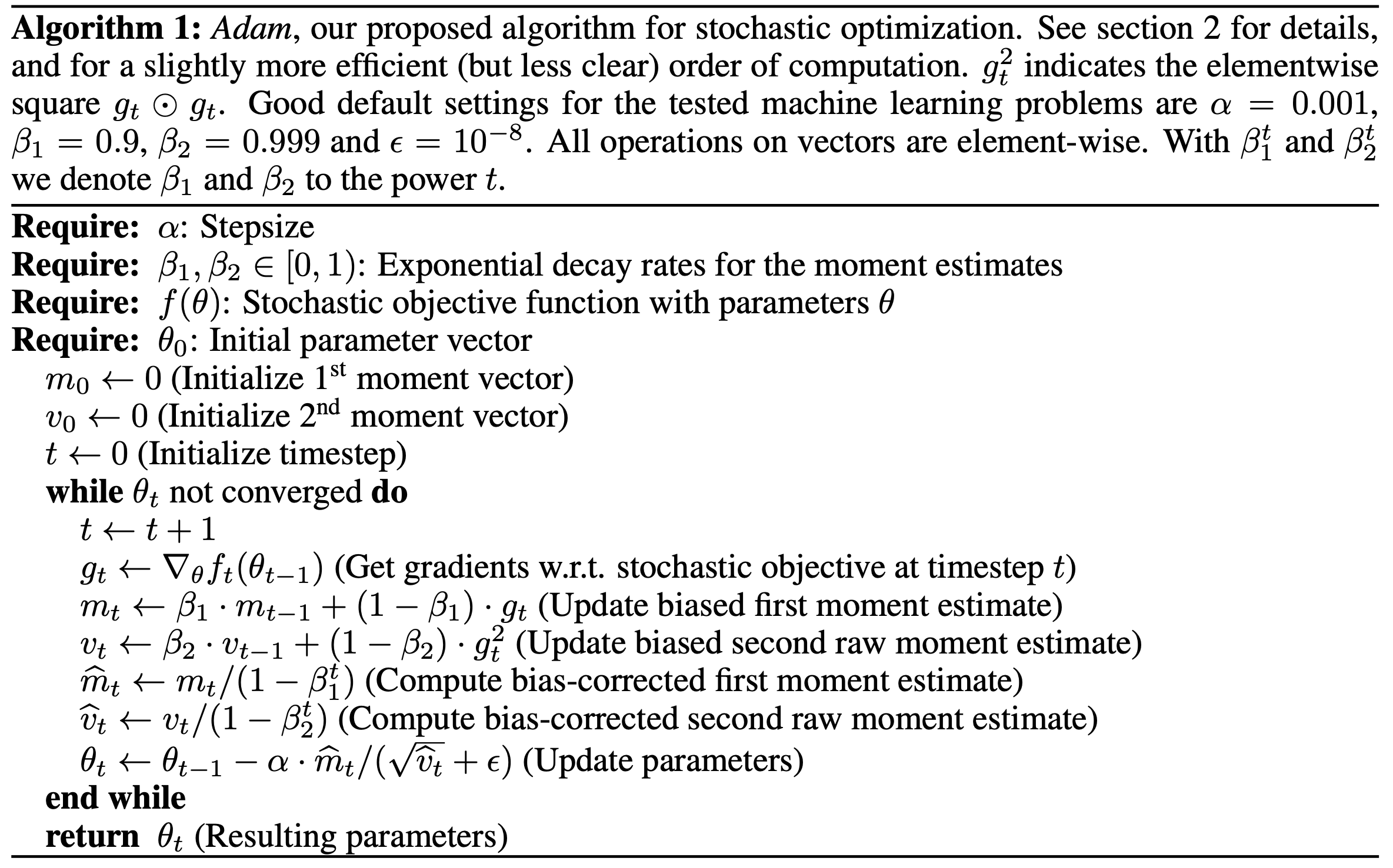
This week's Computer Vision homework has us reading through some ML papers. One of these is Adam: A Method for Stochastic Optimization Kingma & Ba (2015).

Adam is a very widely used gradient descent optimization algorithm that comes as standard in lots of ML frameworks, though recently it's got some competition from the polar Muon algorithm.

Reading the paper, I decided to quickly implement a simple version of the algorithm in Rust to help internalize what it does, and then do a bit of benchmarking.

First Steps

Gonna get into a bit of math here, stick with me.

We can set this up pretty simply as a pure function taking in a handful of hyperparameters: the learning rate (alpha), decay rates (beta1, beta2), a tolerance (epsilon), the optimization function, and the function parameters. We'll be returning the final guess for the optimized function parameters.

After initializing the first and second moment vectors (same length as the parameter vector) we set up the main while loop that runs the program.

Main loop

On each iteration, we're going to:

• Increment the step counter t
• Evaluate the gradient function at the current theta
• Update the first and second moment estimates based on that theta
• Correct the bias in these estimates
• Compute a new theta estimate from those moment estimates

Not quite what I would call simple, but pretty straightforward once it's all laid out.

It's pretty clear to see the orthodox structure of a gradient descent optimizer in here. We're recomputing the moment estimates using a combination of their past estimates and the gradient at the current theta, with the former having a much stronger influence than the latter.

This ratio remains static, but the bias-correction stage is different: as we continue to loop, t increases and the bias-correction coefficients (1-beta1^t and 1-beta2^t) approach 1 (beta*^t approaches 0 as t increases). The further along we get, the less influence the bias-correction stage exerts, as the algorithm assumes that a run that has more iterations under its belt has likely already found something and is unwilling to knock it out of a good-enough local minimum.

So as we continue to loop, we move closer to the local minimum, and become more and more conservative, preferring to consolidate what we have rather than go off chasing the global minimum elsewhere.

Rust implementation

So, how shall we implement this in Rust?

First, let's identify what types we're working on. Our hyperparameters are mainly floating point integers in the [0, 1) range. We can use f64 for these, and either assert their ranges or just trust the user to get it right.

Most everything else, we're going to encode as a Vec<f64>, a heap-allocated vector of floating point numbers. They're all going to be the same size, so we might be able to take this off the heap if we were building this implementation for a very specific use case with a known size for theta, but that loses us a lot of flexibility, and at the sizes of theta we're going to be working with, heap allocation isn't wasteful.

From there, it's going to be a lot of iterating over vectors.

pub fn adam_basic(
    alpha: f64, // stepsize
    beta1: f64, // exponential decay rate for first moment estimate
    beta2: f64, // exponential decay rate for second moment estimate
    eps: f64, // epsilon tolerance
    grad_fn: impl Fn(&[f64]) -> Vec<f64>, // the gradient of the function differentiable wrt its parameters theta
    mut theta: Vec<f64>, // the function parameters
    n_steps: i32, // maximum number of steps before we break regardless of convergence
    convergence_tol: f64,
) -> Vec<f64> {

    assert!((0.0..1.0).contains(&beta1), "beta1 must be in the range [0, 1)");
    assert!((0.0..1.0).contains(&beta2), "beta2 must be in the range [0, 1)");

    let n_params = theta.len();

    // initialize first moment vector
    let mut m_t: Vec<f64> = vec![0.0; n_params];
    // initialize second moment vector
    let mut v_t: Vec<f64> = vec![0.0; n_params];

    for t in 1..=n_steps {
        // evaluate gradient function at current theta
        let g_t: Vec<f64> = grad_fn(&theta);

        // update first and second moment estimates
        m_t = m_t.iter().zip(g_t.iter()).map(|(m, g)| {
            beta1 * m + (1.0 - beta1) * g
        }).collect();
        v_t = v_t.iter().zip(g_t.iter()).map(|(v, g)| {
            beta2 * v + (1.0 - beta2) * g.powi(2)
        }).collect();

        // correct bias in first and second moment estimates
        let m_t_est: Vec<f64> = m_t.iter().map(|m| {
            m / (1.0 - beta1.powi(t))
        }).collect();
        let v_t_est: Vec<f64> = v_t.iter().map(|v| {
            v / (1.0 - beta2.powi(t))
        }).collect();

        // save theta t-1 for comparison
        let theta_old = theta.clone();

        // calculate new theta estimate
        theta = theta.iter().zip(m_t_est).zip(v_t_est).map(|((t, m), v)| {
            t - (alpha * m / (v.sqrt() + eps))
        }).collect();

        // check for convergence
        let distance_sq: f64 = theta_old.iter()
            .zip(theta.iter())
            .map(|(old, new)| (new - old).powi(2))
            .sum();
        if distance_sq < convergence_tol.powi(2) {
            println!("Converged after {} steps", t);
            break;
        }
    }
    theta
}

For the most part, a straightforward implementation, with just a few deviations from the text of the algorithm.

• We implement an n_steps input that allows us to exit after a set number of iterations if we haven't already converged
• We make t the loop counter instead of incrementing it separately, and move to the range of [1..n_steps] rather than [0..n_steps). I can't claim credit for this one: trying to use t as a separate loop counter triggers a compiler warning and linter suggestion, and I think the compiler is right.
• We take in the gradient of the function directly, rather than taking in the function and then computing the gradient. This is mainly for my own convenience, since I wanted to keep this implementation vanilla without introducing other dependencies (also why we're not using ndarray though it would speed things up a lot). We could use the autodiff crate to take in the original function and gets its derivative, but for the time being I'm going to keep things simple for the sake of demonstration.
• We use the L2 norm for checking convergence, but we reorganize the expression to check the square of the distance against the square of the convergence tolerance. This is a micro-optimization that allows us to avoid a square-root operation at the cost of a square, which is favorable: squaring is just multiplication, and that's damn fast, while square roots take multiple operations in succession. The former is just plain faster on modern chips, so any place where you would perform a square root for euclidean comparison (ie you don't need the value itself, just the comparison) it's more performant to just square the other side of the equation.

Some other implementation notes: we save ourselves a .clone() on the moved g_t value at the beginning of the loop by using g_t.iter() instead. This way, both m_t and v_t are constructed from an immutable iterator of references, and we save ourselves some time copying.

Benchmarking Basic Performance

The question you've all been waiting for: how fast is it?

For benchmarking, let's feed it a very simple convex function, f(θ) = Σθᵢ², whose gradient is just ∇f(θ) = 2θ.

Let's also use the suggested hyperparameters in 128-dimensional space, along with n_steps = 100 and a convergence tolerance of 1e-6:

    let alpha = 0.001;
    let beta1 = 0.9;
    let beta2 = 0.999;
    let eps = 1e-8;
    let n_steps = 100;
    let convergence_tol = 1e-6;
    let n_params = 128;

We get the following results from criterion benchmarking:

time: [39.444 µs 39.547 µs 39.645 µs]

About 40 microseconds total, and this increases linearly as we increase n_steps (400 microseconds at n=1000 and 4 milliseconds at n=10,000). That, plus the fact that we don't get convergence statements printed, indicates we're not converging.

This also means we can reliably calculate our inner loop to take around 400 nanoseconds per iteration.

Incidentally, if we didn't drop the .clone() earlier in exchange for the .iter()s, we get around a 10% performance regression, to around 440 nanoseconds per iteration.

Not terrible, but not great. We can do better.

We can get to convergence more quickly by changing the hyperparameters, such as by increasing the learning rate to 0.01, which allows us to converge in around 3700 steps. But what we really want to do is get the individual iteration times down.

Optimized implementation

The biggest optimization we can make from here isn't in the implementation (short of adding ndarray), but rather on the algorithmic side. The original ADAM paper suggests that the basic representation of the algorithm above can be optimized, at the cost of clarity, by replacing the explicit calculation of m_t_est and v_t_est to get theta with the following operations:

It wasn't originally clear why this was an improvement, until I coded it out

        ...

        let alpha_t = alpha * (1.0 - beta2.powi(t)).sqrt() / (1.0 - beta1.powi(t));

        theta = theta.iter().zip(m_t.iter()).zip(v_t.iter()).map(|((t, m), v)| {
            t - alpha_t * m / (v.sqrt() + eps)
        }).collect();

        ...

In the original, we ran through m_t and v_t separately, with a division operation on each item of the iterator. But the denominator is the same every time!

In the optimized version, we're performing just one scalar division to get alpha_t up front, and then running through m_t and v_t together as zipped iterators, using the precomputed alpha_t along the way.

This saves us the overhead and time of a couple short iterators, but also a bunch of divisions (relatively more expensive than additions and multiplications, though still not as expensive as roots).

But how much faster does this actually make us?

time: [29.725 µs 29.810 µs 29.908 µs]

From around 40 microseconds to 30, reliably 33% faster. that's a good speedup right there.

Failed Optimization

I also had my eye on another possible optimization: eliminating intermediate heap allocations in the basic version of the algorithm. That implementation not only allocates m_t and v_t in order to update them, but also collects the results of m_t_est and v_t_est, allocating them separately, even though they're immediately consumed on the next line to calculate theta.

That looks wasteful, doesn't it? And on top of that, it's not even necessary in order to preserve our implementation! If we remove the .collect() call at the end of both of those lines... nothing happens. m_t_est and v_t_est are no longer Vec<f64>, but Map<Iter<'_, f64>, impl FnMut(&f64) -> f64>...

...

Okay, I can kinda see why this makes the language look complicated. I promise it's not that bad! This is an intermediary type produced by using a .map() operation without then collecting the result into a new collection (like a vector, hashset, etc). The resulting type is an iterator, which means we can still plug it right into the .zip(call), since that call would end up turning the collections back into iterators anyway.

This way, we save on the intermediate allocation, and just use the iterators as iterators. Pretty neat.

Now, let's see how much performance... regresses?

time:   [106.78 µs 106.97 µs 107.16 µs]
                        change: [+170.03% +170.78% +171.49%] (p = 0.00 < 0.05)
                        Performance has regressed.

Wow, that is bad.

I'm not completely sure why this is the case. Map<I, F> implements IntoIterator, so that shouldn't be the issue.

My best guess is that, in the original case, the compiler is automatically implementing some SIMD or other vectorization optimizations under the hood, which it can do easily because it's working with the simpler Vec<f64> type for each, but for some reason it is not able to do the same with the Map<Iter> type.

If this is true, it may still be possible to manually implement SIMD on top of the Map<Iter>, allowing us to get that performance boost while still avoiding the intermediate allocations. But that would be a fair bit of work for what is probably a very small performance gain, and would considerably complicate the implementation.

Next Steps

The next step for this would probably be to develop a Python interface using pyo3: but this runs into some blocks, since we need to pass the gradient function into Rust somehow. The number of ML functions used for this isn't especially large, so I could probably just develop several and allow the user to select them via an enum parameter, but that would make this less flexible.